Blog

Here’s my blog. I rant about all kinds of stuff here. When I don’t find time to rant, I tweet.

Opinions are my own.

Quirks of Scala Specialization

posted by Alex,03.11.2013.

Having used specialization a lot and having fixed some of its issues, I came across a couple of useful tricks – I want to document them both for myself and others. Specialization is the feature that allows you to generate separate versions of generic classes for primitive types, thus avoiding boxing in most cases. First introduced in Scala 2.8 by Iulian Dragos, by Scala 2.11 specialization has become a pretty robust language feature, and a lot of its issues have been fixed, but there are places where it might stab you in the back if you don’t watch out. Problem is, specialization interacts with a some edge-cases in the language and obscure language features in ways that are not expected. Sometimes, these are just unresolved bugs. Here are some tips and tricks that might help you.

Note: when used correctly, this is a powerful and extremely useful feature few JVM languages (if any) can parallel these days. Don’t get scared by these tips.

Know the conditions for method specialization

Perhaps you’re not aware of this, but even if a method is a part of a specialized class and contains specializable code, it will not really be specialized unless the specialized type appears in its argument list or its return type. For example:

def getValue[@specialized T]: T = ???

class Foo[@specialized T] {
  var value: T = _
  def reset() {
    value = getValue
  }
}

Above, reset is not specialized. This is an elaborate design decision taken in specialization. If you want reset to be specialized, do something like this:

def reset(): T = {
  value = getValue
  value
}

Be aware that for a method to be specialized, it must either take an argument of specializable type from its environment, or it must return a value of such a type.

But that’s not all. If more than one type-parameter is specialized, then specialized class instances are created only if all the specialized type parameters are instantiated at a primitive type. Here’s a quiz:

class Foo[@specialized T, @specialized S, R] {
  var tv: T = _
  var sv: S = _
  var rv: R = _
}
val x = new Foo[Int, String, String]
val y = new Foo[Int, Long, String]

Will x and/or y refer to a specialized object?

Specialization never generates a specialized class that is a combination of specialized and generic type parameters that have been annotated with @specialized. The compiler will “rewrite” the last 2 lines to:

val x = new Foo[java.lang.Integer, String, String]
val y = new Foo$mcIJ$sp

So, y is instantiated with a specialized class Foo$mcIJ$sp because both T and S are instantiated at primitive types Int and Long, but x refers to a generic object.

Specialization has an all-or-nothing semantics when picking a specialized implementation – all the @specialized-annotated type parameters must be instantiated as primitive types to yield a specialized object.

Don’t be surprised if half-specialized constructor invocations end up creating object instances that box everything. This applies to methods as well as constructor invocations.

Initialize specialized values outside constructor body

Specialization in 2.10 has a problem of specializing constructors in some cases. Lets say you want to track different method invocations until seeing a specific value stopKey and you want your own specialized collections for the task. At some point you could arrive at classes Traversable, Traversable.Buffer and Actions as below:

trait Traversable[@specialized(Int, Long, Double) T] {
  self =>
}

object Traversable {
  class Buffer[@specialized(Int, Long, Double) T]
  extends Traversable[T] {
    def +=(value: T) {
    }
  }
}

class Actions[@specialized(Int, Long) K, V](val stopKey: K) {
  private val insertsBuffer = new Traversable.Buffer[(K, V)]
  private val clearsBuffer = new Traversable.Buffer[Unit]

  def inserts: Traversable[(K, V)] = insertsBuffer
  def clears: Traversable[Unit] = clearsBuffer
}

If you try to instantiate Actions in Scala 2.10.1, you’ll get:

Exception in thread "main" java.lang.IllegalAccessError
  at org.test.Actions$mcI$sp.<init>(Main.scala:57)
  at org.test.Main$.main(Main.scala:21)
  at org.test.Main.main(Main.scala)

I won’t get into why the above fails the way it fails - suffices to say that the specialization creates specialized fields in the specialized variants of the class and does not properly rewire the bridges for the field accessor methods in the constructor body correctly. Here is the pattern to solve the above issues - create a method init in which you initialize the troublesome fields:

class Actions[@specialized(Int, Long) K, V](val stopKey: K) {
  private var insertsBuffer: Traversable.Buffer[(K, V)] = null
  private var clearsBuffer: Traversable.Buffer[Unit] = null
  
  protected def init(sk: K) {
    insertsBuffer = new Traversable.Buffer[(K, V)]
    clearsBuffer = new Traversable.Buffer[Unit]
  }
  
  init(stopKey)
  
  def inserts: Traversable[(K, V)] = insertsBuffer
  def clears: Traversable[Unit] = clearsBuffer
}

Make sure that the init method takes an argument of the specialized type. This will enforce proper specialization and accessing the fields properly. Note that I spent some time minimizing the above example from real, bigger codebase, and it’s not really that easy to trigger it. I won’t get into the precise conditions for this issue to happen, as this is buggy behaviour anyway – the important thing is to know how to solve these kind of IllegalAccessErrors if you run into them.

When initializing more complex specialized classes, consider creating an init method to initialize specializable fields.

Resolve access problems using the `package`-`private` modifier

When you instantiate an anonymous class inside a specialized class and the anonymous class accesses private members of the surrounding specialized class, you might get a compiler error message telling you that the member cannot be accessed. In the following example:

class Buffer[@specialized T] {
  private var array: Array[T] = ???
  def iterator = new Iterator[T] {
    var i = 0
    def hasNext = i < array.length
    def next() = ???
  }
}

an anonymous iterator should have access to the specialized array of the surrounding buffer. Normally, the compiler should remove the private modifier of the surrounding class, so that those fields don’t end up private at the bytecode level (this is the case for both Scala and Java, I believe). With specialization this sometimes does not happen. Solution – just make the problematic members package-private.

Use the package-private modifier for fields meant to be private to resolve access problems in inner classes.

Use `trait`s where possible

For each specialized class C[@specialized T], specialization creates its normal generic version C[T] and a specialized version, e.g. C$mcI$sp, that extends the generic version:

class C$mcI$sp extends C[Int]

and then overrides the bridge methods that need to be specialized. Obviously, extending specialized class C[T] with D[@specialized T] extends C[T] will result in a diamond inheritance and the compiler will drop the specialized C$mcI$sp from the hierarchy of D[T] (you will even get a warning). Dropping the specialized class means you will lose specializations of some methods.

Bottomline is, use traits with specialization if you need to extend specialized classes - they allow multiple inheritance and you won’t lose specialized method versions from the hierarchy.

Use traits in specialized class hierarchies to ensure that all the specialized methods are correctly inherited.

Avoid `trait`s where possible

This seems to contradict the previous hint. Well, traits are problematic. They are not supported natively on the JVM, so the compiler has to generate a lot of bridge methods each time an abstract or a concrete class extend a trait. If you take a look at the standard collections code, there are classes like AbstractSeq which serve no purpose other than to force the compiler to spit out all the bridge methods into a base class like AbstractSeq so that its subclasses don’t have to have all the bridge methods – instead, they inherit them the normal JVM way from this base class, e.g. AbstractSeq. I’ve handwaved the details away here – the important thing is that this technique reduces the standard library size significantly.

Now, thinking in terms of specialization – a specialized method (one inside a specialized class) will have at most 9 bridges for a single specialized type parameter. Obviously, you want to extend specialized traits as least as possible. In many cases you will extend a specialized class only for a concrete type and not for all possible types. A good example are anonymous classes. Lets say you have a trait Observer that observes:

trait Observer[@specialized T] {
  def observe(value: T): Unit
}

You would typically extend it for particular types T as an anonymous class:

eventSource.register(new Observer[Int] {
  var sum = 0
  def observe(value: T) = sum += value
}

Why have Observer as a trait then and generate hundreds of bridge methods everywhere? Instantiate a specialized abstract class AbstractObserver[@specialized T]. Extending it for a single type, e.g. Int, will inherit the specialized variant AbstractObserver$mcI$sp and you won’t lose specialized methods as described in the previous hint.

Use abstract specialized superclasses for anonymous classes and classes extending superclasses with a concrete specialized type parameter to save compilation time and make compiler output smaller.

Make your classes as flat as possible

Specialization is getting more robust, but make no mistakes about it – sometimes it interacts weirdly with some Scala features. Sometimes this is due to bugs, sometimes due to some more fundamental issues.

One important consideration are nested and inner classes. Avoid them! You could write:

trait View[@specialized T] {
  self =>
  def foreach(f: T => Unit): Unit
  def filter(p: T => Boolean) = {
    new View {
      def foreach(f: T => Unit) = for (v <- self) if (p(v)) f(v)
    }
  }
}

Instead, write:

trait View[@specialized T] {
  self =>
  def foreach(f: T => Unit): Unit
  def filter(p: T => Boolean) = {
    new View.Filtered[T](self, p)
  }
}

object View {
  class Filtered[@specialized T](val self: View[T], val p: T => Boolean)
  extends View[T] {
    def foreach(f: T => Unit) = for (v <- self) if (p(v)) f(v)
  }
}

Sometimes the specialization phase of the compiler will fail to reproduce the correct flattening of the nested classes, so you need to do it yourself. The particular example in this hint might even work, but in general avoid nesting specialized stuff in specialized stuff. In the best case, you will receive a warning about some members of the enclosing class not being accessible or not existing.

In general, avoid nesting specialized classes.

Avoid `super` calls

Qualified super calls are (perhaps fundamentally) broken with specialization. Rewiring the super-accessor methods properly in the specialization phase is a nightmare that has not been solved so far. So, avoid them like the plague, at least for now. In particular, stackable modifications pattern will not work with it well.

Avoid super calls.

Be wary of `var`s

Be aware that vars with specializable types may result in an increase in memory footprint. Namely, because of the limitations of the JVM in combination with the current specialization design in which subclasses are specializations of the generic class, the following class:

class Foo[@specialized(Int) T](var x: T)

will result in a generic class Foo with one field x, and a specialized class Foo$mcI$sp with an additional field x$mcI$sp:

class Foo$mcI$sp(var x$mcI$sp: Int)
extends Foo[Int](null)

The original field x is initialized to null in a specialized subclass.

Avoid or minimize vars in specialized classes if memory footprint is a concern.

So what can you do if you still need those vars but want to reduce memory footprint? You can use the following trick. Lets say that you are implementing a closed addressing hash table and need an Entry object for each key. Normally, you’d declare a specialized class Entry with a key field that would be duplicated. Instead, you can declare a trait:

trait Entry[@specialized(Int, Long) K] {
  def key: K
  def key_=(k: K): Unit
}

Now, you can have concrete implementations of that trait:

final class AnyRefEntry[K](var key: K) extends Entry[K]
final class IntEntry(var key: Int) extends Entry[Int]
final class LongEntry(var key: Long) extends Entry[Long]

Each of these concrete entries will have only a single field. To instantiate the correct Entry implementation in the hash table implementation, use a typeclass resolved when the hash table is instantiated:

trait Entryable[@specialized(Int, Long) K] {
  def newEntry(k: K): Entry[K]
}

implicit def anyRefEntryable[K] = new Entryable[K] {
  def newEntry(k: K) = new AnyRefEntry(k)
}

implicit def intEntryable = new Entryable[Int] {
  def newEntry(k: Int) = new IntEntry(k)
}

class HashTable[@specialized(Int, Long) K]
  (implicit val e: Entryable[K])

The most specific implicit is then resolved when calling new HashTable.

Think about the primitive types you really care about

Blindly specializing on all your primitive types is both unnecessary and can boost your compilation times to high heaven, as well as generate thousands of small classes. So, think about which primitive types your application(s) will actually use. I usually specialize on Int, Long and Double, in many cases that’s enough:

class Foo[@specialized(Int, Long, Double) T]

In fact, you will find that the FunctionN classes in the Scala standard library are specialized only for specific types. And the higher the arity, the less they’re specialized.

Restrict your specialized primitive types to ensure shorter compilation times and make compiler output smaller.

Avoid using specialization and implicit classes together

Instead of:

implicit class MyTupleOps[@specialized T, @specialized S](tuple: (T, S)) {
  def reverse: (S, T) = (tuple._2, tuple._1)
}

Do this:

class MyTupleOps[@specialized T, @specialized S](val tuple: (T, S)) {
  def reverse: (S, T) = (tuple._2, tuple._1)
}
implicit def tupleOps[@specialized T, @specialized S](tuple: (T, S)) =
  new MyTupleOps[T, S](tuple)

I’ve ran across situations when specialized implicit classes compiled in a separate compilation run do not pickle the symbols correctly. While this will probably be fixed in the future, if you run into error messages telling you that the MyTupleOps symbol is not available, the above is likely to solve the issue.

Lift expressions to methods to trigger specialization

Remember, specialization of a method is triggered when the all the specialized types are mentioned in the function signature. Consider the following example:

class Source[T, @specialized(Int) S](val event: S) {
  def emit(obs: Observer[S]): Unit = obs.onEvent(event)
  def trigger(x: T): Unit = {
    val obs = new Observer[S]
    emit(obs)
  }
}

class Observer[@specialized(Int) S] { def onEvent(e: S) {} }

Above, in the Source subclass specialized for Int, i.e. in Source$mcI$sp, note that specialized emit, i.e. emit$mcI$sp will note be called. This is because trigger is not specialized, since it does not contain the specialized type S in its signature. This example will box the value event when trigger gets called.

The solution is to lift new Observer[S] to a helper method, which mentions S in its return type.

def newObserver: Observer[S] = new Observer[S]
def trigger(x: T): Unit = {
  val obs = newObserver
  emit(obs)
}

In specialized subclasses of Source, the newObserver method will forward to newObserver$mcI$sp, so trigger itself does not need to be specialized. For user-facing methods, a similar trick is to introduce a fake implicit parameter, just to mention the specialized type parameter.

Parting words

I hope this summarizes some of the useful guidelines when dealing with Scala specialization. I’ll add more tips here if I remember some or run into them.

On the Future of Lazy Vals In Scala

posted by Alex,10.06.2013.

This post has nothing to do with Futures. But let’s cut to the chase. Scala lazy vals are object fields that are not initialized with a value when the object is created. Instead, the field is initialized the first time it is referenced by some thread of control. Here’s an example:

class UnitVector(val angle: Double) {
  lazy val x = {
    println("Getting initialized...")
    math.sin(angle)
  }
}

val v = new UnitVector(math.Pi / 4)
println("Computing x...")
v.x
println("Value of x: " + v.x)

The program prints Computing x. first due to the lazy modifier on x. It prints Getting initialized... only once – after initialization the value is cached, so to speak. Notice the wording “thread of control” above. Indeed, the field x could have been accessed by different threads and as the above example shows, the so-called lazy val initializer block can have side-effects. If multiple threads were allowed to run the initializer block, program semantics would be non-deterministic.

To discard the possibility of executions where the Getting initialized... is executed twice, the Scala compiler transforms the lazy val declarations in the following manner. Assume the following definition:

final class LazyCell {
  lazy val value = 17
}

This is an illustration of what the Scala compiler transforms it to:

final class LazyCell {
  @volatile var bitmap_0: Boolean = false
  var value_0: Int = _
  private def value_lzycompute(): Int = {
    this.synchronized {
      if (!bitmap_0) {
        value_0 = 17
        bitmap_0 = true
      }
    }
    value_0
  }
  def value = if (bitmap_0) value_0 else value_lzycompute()
}

I assume here that you’re familiar with what the synchronized keyword does in Java, otherwise you can think of it as means to lock a critical section.

First of all, there has to be some way of knowing whether the lazy field already got initialized or not. Hence the bitmap_0 field – if it is false, then the lazy val is not initialized, otherwise it is. The space overheads here are negligible – due to object 8-byte boundary alignment, the runtime size of the object will not change on a 32-bit JVM.

Locks are assumed to be (and are) expensive, so it’s not efficient to lock on every read. This is why the bitmap_0 field being annotated as @volatile is being read before acquiring the lock, and is known as the double-checked locking idiom. The lock is only acquired if the bitmap_0 is false, implying nothing about whether value_0 was assigned, so a thread might try to acquire the lock of the LazyCell object and execute the initializer block, in this case just 17. However, reading bitmap_0 guarantees that value_0 was assigned, in every execution. To see why this is so, search around for the Java Memory Model and the volatile semantics. Bottom line – if you understand the transformation above, you understand how the lazy val initialization works in Scala, and should be convinced that it is safe.

Or, should you?

As some people in the Scala community recently remarked, this can lead to some pretty weird behaviour. The following example should work perfectly:

object A {
  lazy val a0 = B.b
  lazy val a1 = 17
}

object B {
  lazy val b = A.a1
}

Should it? Does it? Or not? Try to see why.

Unfortunately, if A.a0 is accessed by some thread Ta and B.b is accessed by some thread Tb, there is a possibility of a deadlock. The reason lies in the lzycompute method shown earlier – both threads attempt to grab a hold of the other object’s lock from within the initializer blocks of the lazy vals a0 and b, respectively. While doing so, they do not let go of their own lock. Thus, a deadlock may occur when using several lazy vals referring to each other, although they do not form a circular dependency.

This problem is more serious than it may seem at first glance – patterns that address initialization order issues use lazy vals and some Scala constructs are expressed in terms of them, nested singleton objects being the most prominent one.

Better Lazy Vals

We attempt to categorize and address these issues in SIP-20, a Scala improvement proposal available at the docs site.

The basic idea behind the proposed changes is very simple. Instead of selfishly holding the lock of the object containing the lazy val, the lock is acquired once to let the other threads know that some thread is initializing the lazy val, and once more to let them know that the initialization is completed. The threads that arrive after initialization has started but before it has finished are forced to wait for completion on the monitor of the this object.

Here as an illustration:

class LazyCell {
  @volatile var bitmap_0: Int = 0
  var value_0: Int = _
  private def value_lzycompute(): Int = {
    this.synchronized {
      if (bitmap_0 == 0) {
        bitmap_0 = 1
      } else {
        while (bitmap_0 == 1) {
          this.wait()
        }
        return value_0
      }
    }
    val result = 0 // the initializer block goes here
    this.synchronized {
      value_0 = result
      bitmap_0 = 3
      this.notifyAll()
    }
    value_0
  }
  def value = if (bitmap_0 == 3) value_0 else value_lzycompute()
}

Note that this new scheme requires more than 2 bitmap states, but this does not change the memory footprint significantly and in most cases not at all.v

We explore several variants of this idea in the SIP, and state the perceived advantages and disadvantages of each. The SIP also comes with a solid suite of microbenchmarks, designed to validate the assumption that the lazy val performance will not change significantly.

Beyond Lazy Vals

And now the point behind this blog post – the proposed scheme does not solve all the lazy val issues. Since this scheme relies on acquiring the monitor of the this object, it will fall short in some interactions with the user-code. Here’s an example from the SIP:

class A { self =>
  lazy val x: Int = {
    (new Thread() {
      override def run() = self.synchronized { while (true) {} }
    }).start()
    1
  }
}

If the newly created thread starts running before the caller thread acquires the monitor in the second synchronized block, a deadlock occurs. More subtle and more realistic scenarios can likewise cause deadlocks. The SIP does not address them.

Ideally, a basic language feature like lazy initialization should address these issues, which might render it a leaky abstraction. There are some solutions, but there are also reasons why they are not in the SIP.

As few people have suggested, there exist initialization schemes not mentioned in the SIP that avoid deadlocks due to interactions with the user code. Since these interactions are due to user code synchronizing on the same object as the behind-the-scene lazy val initialization mechanism, a solution is to make the lazy val initialization mechanism synchronize on some other object. A compiler could emit a hidden dummy object field and initialize a dummy object for each lazy val, so that initializing threads can synchronize on it, but the user code cannot see it. Something like this:

class LazyCell {
  @volatile private var bitmap_0 = 0
  @volatile private var value_dummy = new AnyRef
  private var value_0 = _
  private def value_lzycompute() = ??? // sync, init, sync
  def value = if (bitmap_0 == 3) value_0 else value_lzycompute()
}

This is an overkill – on average it increases the object size by 12 bytes per a lazy val field on a 32-bit JVM. So lets try something smarter. Instead of creating many objects and fields for them, we could have a single field for all the dummy synchronization objects used at one particular instance in time stored in an immutable list. While the list would be immutable, the field for the list would be volatile and modified with a CAS. Given a class:

class A {
  lazy val x = 17
  lazy val y = 19
}

here’s one possible scenario for such a list, where y is initialized first and x after that. Dummy synchronization objects are removed from the list once the initialization fully completes and the corresponding bitmap entry was updated.

list --|
list --> [ y ] --|
list --> [ x ] --> [ y ] --|
list --> [ x ] --|
list --|

This might have more runtime overheads than is reasonable, though. The prospect of having to traverse this list when there are multiple lazy vals is particularly unsettling to me. It also does more bookkeeping at runtime than is actually necessary. Read on.

An alternative to this lock-free scheme that seems to have a lot of runtime overheads is to keep one object per lazy val field in the companion object of the class. Comparing this approach with keeping a concurrent linked list, it scales field-wise, assuming that the false-sharing issues are handled correctly, but does not scale instance-wise, since all the threads initializing the same lazy val field of different objects would access the same dummy synchronization object. But, we could have multiple dummy synchronization objects in the companion object. Threads that initialize a lazy val field could choose one uniquely based on the object’s identityHashCode value.

object A {
  val x_dummies = Array.fill[AnyRef](N)(new AnyRef)
  val y_dummies = Array.fill[AnyRef](N)(new AnyRef)
}

This seems better than the list approach, because it only allocates the dummies only once. Also, the number of threads causing contention on the dummies at a single point in time is at runtime bound by the number of processors. And indeed, by tweaking the N and relating it to the number of processors P we can decrease the probability of contention on a dummy synchronization object arbitrarily, although N grows quadratically with P for a fixed probability – see the birthday paradox.

A downside common to the last two schemes is that they rely on using CAS. As soon as the @volatile bitmap is written to outside of a synchronized block, CAS with retry logic cannot be avoided, since there might be lazy val fields in the same object being initialized concurrently. We discuss in the SIP what using CAS entails.

In conclusion, solution to the lazy val initialization problems should be:

simple - because simple is easy to implement
simple - because simple often means efficient
robust - work in all theoretical scenarios
robust - work in practical circumstances

Looking back at the hypothetical solutions above, although they in theory solve the user code interaction issue, none of them works in practical circumstances well (using CAS might be problematic, and false sharing issues are not immediately apparent), is probably not too efficient in the common case (although this wasn’t tested) and could be too complex to understand, implement or maintain.

But if I had to choose, I’d pick the one with the dummy synchronization objects in the class companion object. Seems to be the simplest and is scalable both field-wise and instance-wise.

Isometric Scala Game Engine

posted by Alex,20.04.2013.

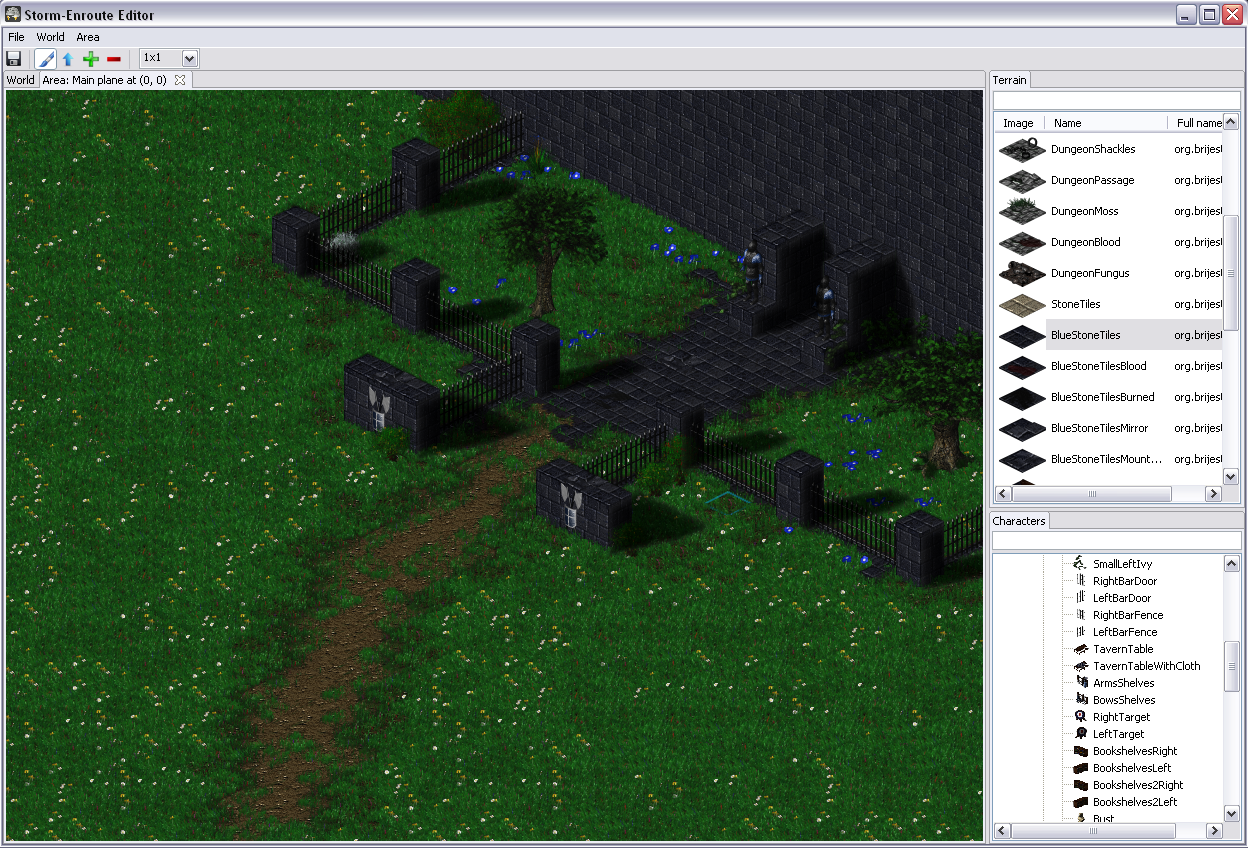
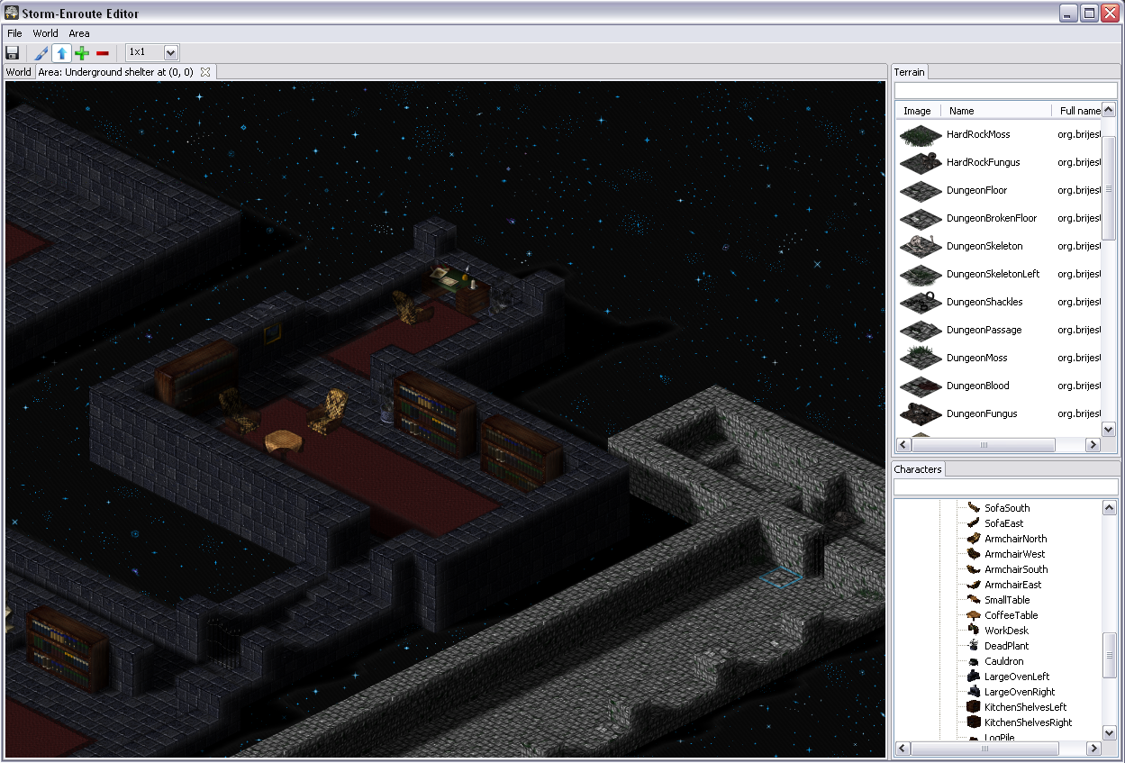
Last year I’ve spent some time working on an isometric RPG-like game engine written in Scala. Knowing that I wouldn’t be able to write a game in my free time alone, I’ve decided to limit myself to a level editor rather than a complete game.

One of the classic arguments people have against Java when it comes to coding games, and along that line Scala too, is bad performance – I was eager to find out to which extent this is really a problem. While what I wrote is not a Crysis engine and this is hardly an extensive analysis, it seems to me that with a little knowledge of what certain higher abstractions translate into, you can write fairly efficient game engine code when it comes to Baldur’s Gate/Diablo style RPG-like engines. The level editor is written largely in Scala, relying mainly on SWT and OpenGL libraries (specifically, the JOGL bindings), with a little bit of shaders written using GLSL. There are some screenshots below.

</img>	</img>
</img>	</img>

In case it’s not obvious from the screenshots – I am a huge fan of sprites. You can’t blame me – I grew up on them. In fact, I am one of those guys who believe that stunning graphics is not an essential ingredient of a quality game or a prerequisite for good gameplay. In fact, I spent a lot of time playing games like ADOM. A bit of nice visual effects is fine, but the game should not be just about those. Also, sprites often allow a higher level of detail, which is neater to the eye. This higher level of detail comes from the fact that they are pre-rendered, potentially using models with a higher polygon count, special effects like hair and fur, as well as material models that allow defining surface properties such as reflection, bump and transparency. Although GPUs are getting faster every day, usually it is more expensive to compute these on-the-fly. But, I will get back to this at the end of the post.

However, this blog post is not meant to be a philosophical debate – rather, I want to share some of my experience of implementing in Scala. In the rest of this blog post I describe the details of the engine implementation. I will go through the rendering process, some of the advantages of Scala when it comes to conciseness and pretty code (particularly when dealing with OpenGL) and creating sprites using 3dsMAX with some custom MaxScript functionality for outputing data for 3d objects. Finally, I share some thoughts on what I would do differently, what some of the goals were and possible future work if my free time allows it.

The rendering procedure

As mentioned before, most of the game is sprite-based. All sprites are rendered using 3ds MAX and then placed into appropriate positions by the game engine at runtime to produce the entire image. What are sprites? In short, these are two-dimensional images integrated into a larger scene. The scene is in this case what you see in the screenshots above. A sprite is just a relatively small PNG image with transparent background that you can blend into the scene. 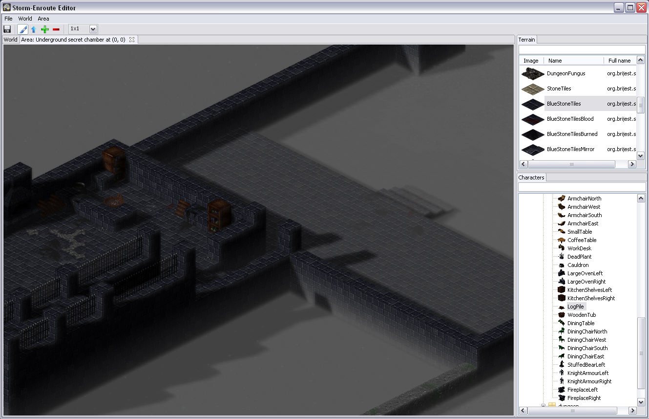There are two basic types of sprites in this engine. The first are terrain sprites and the second character sprites. The fireplace shown on the right image is a character sprite – it is rendered above the terrain sprites. The small rhomboid on the left with some grass on top is a terrain tile. Terrain tiles cover the scene – other sprites are rendered to appear as if they are above them. Terrain tiles are sprites that have a fixed size, whereas character sprites may have a different height and may occupy several tiles.

When it comes to fully 2D top-down perspectives it’s very easy to place sprites into the scene – usually it amounts to passing through the image in the order in which sprites should appear and blending them. In the case of tile-based top-down perspective games, where different sprites occupy different tiles, this means having to loop through the rows of tiles in the scene and through the tiles in each row. However, when it comes to isometric tile-based engines where a sprite may occupy more than a single tile, things get a bit more convoluted. The chair on the left occupies a single tile (1x1 sprite), but the oak tree on the right occupies four tiles (2x2 sprite) and the fireplace shown earlier occupies three tiles (1x3 sprite). The sprites can no longer be drawn going from one corner of the scene to another, so two simple for loops will not do. 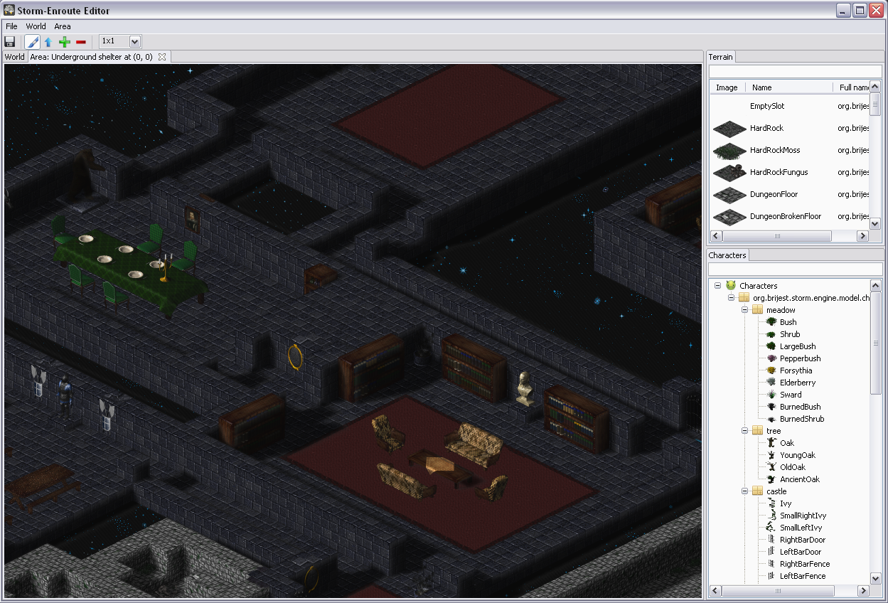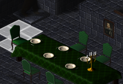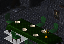Lets focus on the following detail in one of the screenshots – a dining table with chairs around it. 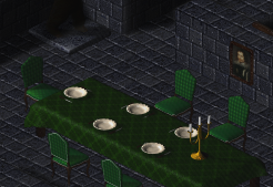The dining table is something like a 7x3 sprite and each chair is a 1x1 sprite. If we render rows of tiles from the north-east going to south-west, and render tiles in each row going from north-west to south-east, then the chair on the head of the table will be rendered after the table, making it seems as if they overlap. Consequently, if we render the rows from north-west to south-east, then the chairs in the middle of the table will be drawn over it.

The naive approach of sorting all the visible sprites in the scene (either by maintaining a binary search tree or sorting them just once before rendering) and then rendering them in that order won’t work either. The problem is that the sprites that occupy rectangular areas do not form a total order with respect to rendering (note that the more general problem of rendering sprites that occupy non-rectangular areas is not really solvable – in this case sprites could overlap). Instead, they form a partial order – given two sprites and their locations on the screen you can only tell which should be rendered first if they overlap. Otherwise, their relative rendering order depends on other sprites that are potentially between them. This means that binary search trees or an efficient comparison sort won’t help you. These approaches assume the existence of total order between the elements, without it the sprites would be spuriously rendered out of order.

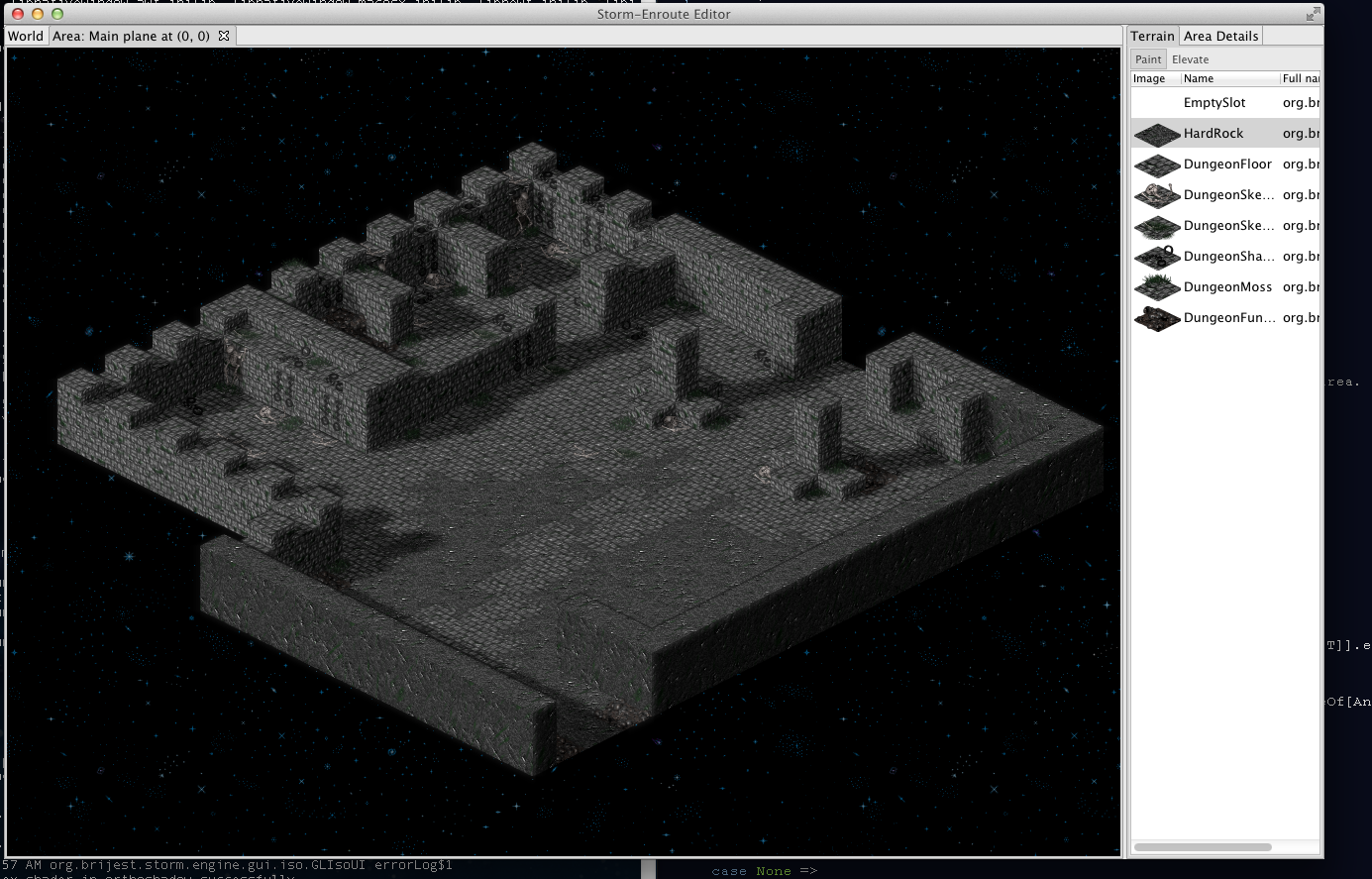
Another complicating factor is that the terrain is not just one huge flat area – different terrain tiles can have different elevations. This design decision is meant to make the whole scene more realistic. Note, that the engine does not allow two tiles to be above each other, though, to keep things simpler.

After having shown the difficulties of rendering in an isometric tile-based scene, lets show how our engine copes with this. First of all, notice that while a classic comparison sort requires the elements to form a total order, comparing all the elements of the scene mutually can yield a proper rendering order (this is precisely what efficient comparison sorts were designed to avoid by relying on the transitivity property of the total order). We can compare each sprite X in the scene to each other sprite Y in the scene and store a dependency X->Y if Y should be rendered before X. This forms a directed acyclic graph (we have to be careful how exactly we define dependencies between sprites to guarantee this acyclicity). To render the sprite X we can then find all the sprites Y for which there is a dependency X->Y, and recursively render sprite Y if it has not been rendered yet – only after all the dependencies have been rendered can X be rendered itself. Unfortunately, this also yields and O(n^2) asymptotic complexity when creating the dependency graph as the number of sprites n grows, which will typically happen as the screen resolution goes up.

However, it is straightforward to see that we do not need to look for a dependency between all the sprite pairs. Most of the sprites have the property of being relatively small, so the sprites that they could overlap with should be somewhere in the immediate vicinity. In the image on the right the tiles that could contain sprites that the chair could possibly overlap with are highlighted. Note that we have to check only 7 tiles for objects instead of thousands of them. In this case there are no objects “behind” the chair, so it has no dependencies. On the image on the left we highlight the tiles the second chair depends on – in this case those tiles contain the dinner table, and the chair has a direct dependency on it. The dinner table on the other hand has a dependency on the first chair, so there exists a transitive rendering dependency between the second and the first chair. Once the dependency graph is fully created a simple for-loop can be used to render all the tiles and the sprites on the screen by checking if all the dependencies have been rendered and rendering them when required. Note that in the worst case the complexity is still quadratic, but only if all the sprites have sizes proportionate to the size of the screen, and no sprites are that big.

Note that each sprite has multiple dependencies – this means we cannot tightly encode all the dependencies within a single object, because there is a variable number of them. We could use a dynamically growing array to store the dependencies, but then we have to dynamically reallocate the array and copy dependencies. We could use linked lists to avoid this, but allocating a node for each link increases the memory footprint, the amount of work and also creates a pressure on the garbage collector. Instead, we use something in between arrays and linked lists – an unrolled linked list. Instead of each node holding a single dependency, it holds several of them, in our case up to 32. Once a node is filled, an additional dependency node is allocated. We encode this as follows:

final class DepNode {
  val deps = new Array[Int](32)
  var sz = 0
  var next: DepNode = null
  var freeNext: DepNode = null
}

The deps array contains the dependencies for the current sprite encoded as tile coordinates, while the sz field denotes how many entries in the array deps should be considered – the array may not be full. Adding a new dependency amounts to writing to the array and incrementing sz. Once sz is equal to 32 we allocate a new DepNode object and assign it to next. We will come back to describing what the freeNext field is used for. To traverse all the dependencies, we have to traverse the deps array, and the next node recursively if it is non-null. This way the unrolled linked list traversal performance can be made arbitrary close to that of a regular array traversal, and it has nice locality properties as well.

Interestingly, while this decreases the memory footprint on the JVM, the actual performance difference between unrolled linked lists and regular linked lists is not that big. This is partly because the GC has to do approximately the same amount of work when collecting the unrolled linked list nodes as linked list nodes, and partly because each time an array for the unrolled linked list is allocated, it has to be cleared first. Although object pooling on the JVM is generally not recommended, we can avoid these two costs in this case by maintaining a variant of a free list memory pool implementation. We maintain a separate singly linked list of DepNode objects, linked together using the freeNext field. To allocate a DepNode object we do the following:

var freeList: DepNode = initialPool()

def alloc(): DepNode = {
  if (freeList == null) new DepNode()
  else {
    val depnode = freeList
    if (depnode.next == null) {
      freeList = depnode.freeNext
    } else {
      depnode.next.freeNext = depnode.freeNext
      freeList = depnode.next
      depnode.next = null
    }
    depnode.freeNext = null
    depnode.sz = 0
    depnode
  }
}

Essentially, we create an object if there are no free objects left in the free list. Otherwise, we return the first object on the free list. If the first object had its next field set to null, then the free list head becomes the next object in the free list as denoted by the freeNext field. Otherwise, the next node in the unrolled list that depnode was previously a part of becomes the head of the free list.

Once the frame is rendered, all the sprites in the scene have to have their dependency lists deallocated by calling dealloc. Keeping a two-dimensional free list like this makes the deallocations really fast:

def dealloc(depnode: DepNode) {
  depnode.freeNext = freeList
  freeList = depnode
}

Not having a two-dimensional free list would require deallocating every unrolled linked list node by traversing the list, and O(n) operation for each list – although most sprites will not have many dependencies, this would still be slower.

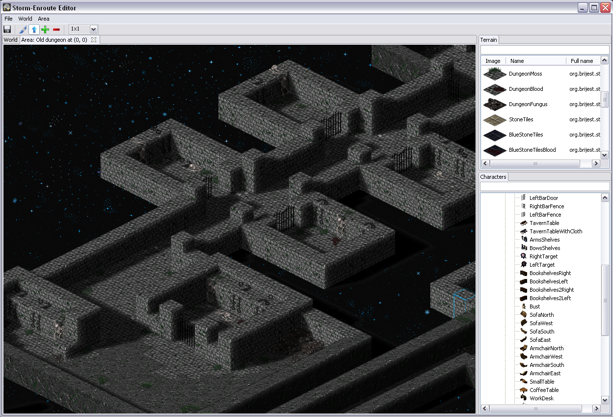
Once all the sprites are rendered we end up with a nice-looking scene, although somewhat flat. Such a scene will be lacking depth – if you played Crusader in the 90s you’ll know what I’m talking about. To overcome this and add more realism, we do something untypical for most sprite-based engines – we employ shadow-mapping so that the objects cast shadows. Shadow-mapping is a technique that requires a 3D representation of the scene, which the sprites lack. In the next post in this series I will describe how we achieve shadow mapping.